A real world check on climate model calculations of atmospheric radiative forcing
Interview with Chris Rentsch
by Paul Huber
Computer climate models make projections of the future using the best assumptions and calculations of how the climate system works. But relying on them requires that we
check them against the best real world data available.
Max Planck is considered one of the founders of quantum mechanics for his discovery of the Planck constant, a quantum unit which reconciled the difference between the theoretically predicted
and observed thermal spectrum of an object. In 1903 he published a book titled “Treatise on Thermodynamics” and in it he explains that matter and objects can transfer thermal energy through
conduction of thermal motion or transmission of thermal radiation.
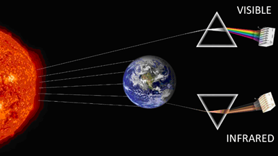
Because Earth exists in the relative vacuum of space, not in contact with anything else, it can only transfer thermal energy radiatively. It’s heated by the Sun’s radiation and gives off its
own thermal radiation in the infrared spectrum. The gaseous atmosphere between the Sun and Earth’s surface interacts with that electromagnetic radiation, reflecting it, absorbing it, and
emitting its own. Its own emission, in the form of downwelling infrared light, is what some call the greenhouse effect. Though it’s an imperfect analogy, because the physics are different,
it can serve a useful purpose in discussing Earth’s energy balance between incoming and outgoing radiation. CO2 is considered a greenhouse gas because it’s infrared-active,
both absorbing and emitting infrared light. That’s why it’s important to understand its effects in the atmosphere in an accurate way.
(Q0) Some of the gasses in the atmosphere are infrared-active, meaning they absorb and emit infrared light. What is it about the physical structure of the CO2 molecule that
makes it IR-active and why is its absorption selective within the spectrum of outgoing IR?
(A0) There are two physical laws that produce the coincidental overlap between CO2's absorption and Earth's emission: Planck's Law (left) and Hooke's Law (right):
Planck's law establishes the range over which an object emits IR at a given temperature. Earth's distance from the sun largely sets the surface temperature and we see that at Earth's
average temperature, 288K, the CO2 v2 band is almost dead-on top of Earth's peak infrared radiance. If the Earth were 200K or 500K instead of 288K, CO2's effect would be
much less pronounced as it would land on the shoulder of the infrared emission peak.
But what causes CO2 to absorb so strongly at 668 cm-1 in the first place? We know that skyscrapers of various heights wobble when an earthquake strikes and those whose
vibrational tendency happens to match the earthquake's vibrational frequency are most likely to collapse. This matching of the input frequency to the structure's natural frequency is called
a resonance and the magnitude of wobble gets larger and larger until the building collapses. Something is similarly true for CO2 molecules and photons:
- We can think of CO2 as a ball-and-spring object which is a simple harmonic oscillator.
- A photon is a wave and a particle simultaneously. In this case, we are more interested in its wavelike behavior, which has a single characteristic wavelength and frequency.
If the frequency of the photon wave packet striking a molecule matches the natural resonant frequency of a molecule's ball-and-spring vibration mode, the photon is likely to be absorbed.
It is also likely that the vibrations of the molecule will emit a photon at some point. More photons are emitted if the gas is warmer, fewer photons if it is cooler. The photon of emission
will be at a wavelength that matches one of the many vibrational modes, but does not necessarily match the vibrational mode of the photon that was absorbed. If a photon of a different
wavelength is emitted, the difference in energy remains in (or is deducted from) the molecule's temperature, in perfect conservation of energy.
CO2 has three vibrational modes: symmetric stretching, asymmetric stretching, and bending (images here).
Using Hooke's law and plugging in the masses of carbon and oxygen, one can derive the v3 asymmetric stretch absorption frequency (example math
here). You can't use Hooke's law to derive the critically important v2 bending absorption frequency,
but there are more advanced mathematicians that have provided walkthroughs. Incidentally,
nitrogen and oxygen have fewer absorption frequencies because, having only two atoms, oscillate in fewer different ways. Nitrogen atoms have a triple bond, which tightens the spring and makes
the wavelengths of active absorption shorter.
Therefore, as a natural consequence of the carbon dioxide molecule having bonds that act like springs and atoms that act like spherical masses, the molecule is capable of vibrating at
specific frequencies that make it particularly capable of absorbing photons at 668 cm-1, a wavenumber that coincidentally matches Earth's primary IR emission wavenumber given
its temperature.
(Q1) What caused you to take up this study?
(A1) I imagine like many others, I heard exhortations to change my lifestyle via article headlines and news sound bites quoting Al Gore’s catastrophic predictions
of an ice-free arctic by 2020 and variations of “we have only 7 years to take action”. These had a certain inconceivability to them, but I couldn’t necessarily explain precisely why.
I had formal training in mass and energy balances, including convection and radiation, so I had some sense of the energy requirements to melt thousands of square kilometers of ice (enormous)
and I knew the effect of adding an absorbing gas to the atmosphere exponentially declines, so each incremental unit is tinier than the one before it. I would later learn Danny Kahneman
describes this as having a ‘strong’ intuition, in contrast to a ‘clear’ intuition.
But, I was assured my skepticism would easily be resolved by a confirmatory time-series infrared radiation measurement of CO2 forcing in models. Not the kind of infrared measurement you
receive when someone takes your forehead temperature with an IR gun; those are broadband detectors that record IR at all wavelengths between 8-12 μm. Rather, the causal link between global
warming and CO2 requires spectrophotometric IR analysis, which means dividing up the IR into its individual colors (via prism or diffraction grating) and measuring the change specifically
at the wavenumbers absorbed by CO2.
The problem was, the study didn’t exist. This was almost inconceivable to me, after all, there is a lot of money going into climate research. The ten largest economies have major
climate modeling efforts underway. CMIP6 alone has >500 contributing researchers operating >12 supercomputers. There are about a hundred thousand climate change studies published each year,
some things as minor as the climate effects on one parasite on one mollusk in one ocean (not making this up). Where was the core, fundamental study experimentally verifying that higher
CO2 produces the expected reduction in outgoing infrared radiation?
The paper didn’t exist, which left me with a choice: join a chorus of critical voices and announce no such study existed in an attempt to drain some of the “certainty” out of
catastrophic claims or create the missing study. I read Montford’s book on the McKitrick/Macintyre vs Mann saga and it actually taught me an important lesson: No one can successfully
attack a study, you can only replace it with something superior. That is, people don’t listen to detractors unless the critic has a better, more-credible offering. In my opinion, MM should
have published their own temperature reconstruction using all of the available tree rings (not just 5%) and their version of a principle components analysis (no centering). Then they would
have provided the world with an alternative to MBH98. Correspondingly, if I wanted to tell the world that CO2 forcing behind the climate alarmism is strictly from computer models, my
expectation was “nobody will care,” unless it could actually be shown by satellite measurement how far the computers were in error (if at all). I also knew that I personally had to bear the
entire cost of the project because anyone even slightly criticizing climate change science will have their funding record scrutinized to find out “whose pocket they are in.” I thought at the
time this would cost <$300, but so far, the cost of programmers and external hard drives has run north of $2,000. If my paper is accepted to an open access journal, it will cost another
$1,800 to publish. I didn’t know authors paid to have their work published, I thought that was what subscribers did. People have offered to contribute, but I continue to turn them down.
(Q2) You state at the beginning of your paper that you chose the AIRS satellite because it had the longest observational record. Was it an easy choice or did the other systems
offer advantages that made it difficult?
(A2) AIRS was engineered to operate for a minimum of five years and now it’s been going strong for over eighteen. It would actually have been an uninteresting dataset if it were only
five years. The two instruments that came before AIRS each operated for less than 11 months, so it is fantastic that AIRS has held up for so long. The instruments launched after AIRS are
actually higher resolution – IASI is about 4x higher and is probably a superior instrument, but it hasn’t been in orbit long enough.
Previous studies from Harries and Brindley attempted to compare spectra collected by IRIS-D and IMG 25 years apart, but a quantitative comparison between two different detectors with
two different resolutions, diffraction mechanisms, and fields of view requires too many mathematical compensations to result in a quantitative forcing estimation.
There is an activity underway to produce a merged multi-satellite dataset that provides a continuous, uninterrupted OLR spectral record. This is an important effort because perhaps
after 25-30 years, AIRS will de-orbit and conclude useful data production. It needs to be joined up to the next satellite(s) and I think within the next ten to twenty years this could become
the most valuable dataset that climate science has.
(Q3) To get the truest signal you wanted to avoid the influences of clouds and daytime solar radiation. How significantly would they have affected your measurements?
(A3) Clouds are effective reflectors and absorbers of longwave infrared. You can see this in CERES measurements where Africa is emitting 300-380 W/m2 but when a cloud
passes by, OLR drops to 50-150 W/m2:
can also see the strong effect of clouds in ground-based AERI measurements. When a thick cloud passes overhead in the Southern Great Plains (SGP), the total downwelling IR, as measured
by the total area under the red curve, goes up about 4x compared to clear-sky downwelling IR, as measured by the total area under the blue curve. This is Earth’s IR reflecting off of the
bottom of the cloud back toward the surface.So, a stratocumulous cloud can reduce the outgoing IR by ~75%. If such a cloud blocks more of the tropics in 2003-2005 than it does in 2016-2018,
this would induce a positive trend bias.
(Q4) Over the observational time period, you’re looking at a relatively small change in radiative forcing and it has to be calculated as accurately as possible. A major factor
to deal with is the Planck response, or feedback, where a warmer surface emits more thermal infrared. As an example, a difference in Earth’s surface temperature from 280K to 283K would yield
an additional ~15 W/m2 (at 0.97 average emissivity) of infrared from that surface. How do you adjust for the Planck response?
(A4) The way I interpret this question is: “How do you measure forcing accurately when the surface temp is variable and the regions where the atmosphere is partially-transparent are
emitting variable, but generally increasing, amounts of infrared radiation? The answer is: I don’t, because when I compare to computer models, I always compare to effective radiative
forcing (ERF). This forcing value tends to be about 18-20% lower than RF because it includes the bit of increased OLR in response to additional RF.
(Q5) The change in radiative forcing seems to be primarily at the wings (sides) of the CO2 absorption band and not at its center. Is this due to
the band saturation effect?
(A5) I would encourage everyone to play with an online line-by-line radiative transfer model (LBLRTM) such as the one here:
http://climatemodels.uchicago.edu/modtran/ Take out all of the greenhouse gasses except for CO2, then slowly
add CO2 back in starting at 0.1 ppm and increasing by a factor of 10x.
The top-of-atmosphere IR emissions drop, but they don’t go to zero: they reach the radiance that corresponds to the temperature of some higher level of the atmosphere. Interestingly,
this can actually lead to higher IR emission at, for example, 668 cm-1 when the elevation of emission climbs up into the stratosphere. The ozone in the stratosphere absorbs enough UV to warm
the upper atmosphere, so higher levels of CO2 can elevate the IR emission into this warm layer.
(Q6) AIRS does not measure the lower wavenumber side of the absorption band, because of instrument limitation, so your values are based on a presumption of symmetry of the band
and you double the other side to account for that absence. Is the symmetry because a resonance response curve is symmetrical?
(A6) Essentially yes. You can see the symmetry mirrored at 668 cm-1. Lines are actually 1.1-1.3x stronger on the higher wavenumber side, but the range of strengths over
which CO2 absorption lines vary is about six orders of magnitude, so 1.1-1.3x is relatively small.
(Q7) Two other factors can also affect the absorption band: atmospheric pressure broadening and Doppler shifting, where motion of the gas molecules slightly changes the relative
frequency of the IR acting on them. Would these factors also be symmetrical?
(A7) These factors are primarily of concern for the people modeling atmospheric emission, not those measuring atmospheric emission. To accurately reproduce the infrared
emission from a given altitude at a given wavenumber, the pressure and temperature at every altitude should be known. Higher temperatures will decrease the absorbance line strength at some
wavenumbers (band centers) and increase the absorbance strength at band edges. So, accurate temperature vs altitude is required. However a satellite detector makes no special calculations,
it simply measures what arrives at the sensor, regardless of the altitude, pressure, or temperature of the emission location.
The day I learned about pressure broadening, Doppler broadening, and temperature adjustments to line strengths galvanized my resolve to obtain empirical measurements. I could not imagine
global circulation models accurately calculating these adjustments:
… for these 142,831 CO2 v2 band absorbance lines:
I would later come to learn that, indeed, GCMs do not even attempt such calculations (far too computationally burdensome) and instead rely on vastly-simplified parameterizations.
What inaccuracies might this introduce? I wanted to see model-measurement comparisons to find out.
(Q8) You mention that doubling the measured wing likely yields a conservative (higher) value since the unmeasured wing overlaps with water vapor absorption and is likely a bit
less as a result. Could you elaborate?
(A8) Water vapor absorbs IR extensively in the far infrared (the longest wavelengths which are the smallest wavenumbers, <650 cm-1). Humidity is primarily confined to the
troposphere, the lowest 10 km of an ~80 km atmosphere. Depending on the humidity levels, the surface IR emissions may be significantly absorbed before interacting with CO2 in the
atmosphere 10-80km up.
I am working to compare AIRS measurements to model calculations and there is one particular latitude band where the model-measurement agreement is quite good. If we look at the model’s
calculation of the humidity-affected wing, we do indeed see it is slightly smaller than the measured wing (see above left video).
(Q9) Instrument viewing angle is important to getting an accurate measurement. You refer to Lambertian emission of the Earth’s surface and isotropic emission of atmospheric
gasses. Could you briefly explain the differences?
(A9) We most commonly encounter the surface descriptor “Lambertian” when describing reflective surfaces. Unfinished wood and coal have a textured surface that imparts a
directionally-universal reflective property. Shiny surfaces do not have this same directionally-universal appearance as they can produce specular reflections.
In my manuscript, I use “Lambert” or “Lambertian” in a less commonly-encountered mode referring to surface infrared emission. Not all surfaces qualify as Lambertian emitters, but I
cannot yet comment on the whether the trees of a pine forest or the wavy ocean surface is the better Lambertian emitter.
“Isotropic” is used more on books that describe emission from a cloud of gas molecules. Isotropic essentially means “equally in all directions.” So, a gas cloud emitting infrared
radiation isotropically has no directional preference. This makes good sense as we really wouldn’t expect a uniform parcel of gas to have major and minor emission axes.
(Q10) What empirical checks on mathematical modeling would you like to see in the future?
(A10) When I started this project, I was under the impression that CO2 radiative forcing was the primary heating mechanism underpinning global warming. In fact, the IPCC
reports indicate that CO2 slightly warms the atmosphere, lofting more water vapor skyward. The assertion is CO2 forcing is amplified 2-3x, making CO2 forcing
the minority effect. This in turn triggers a cloud response adding even more forcing (this all according to climate models, which don’t agree with each other on the magnitude or direction
of the knock-on effects). Thus, a great deal more (4x+ more) radiative forcing is attributed to CO2 than just CO2’s direct effects. Empirical checks are needed on
the feedback responses, and they are 4x more important than the direct effects of CO2.
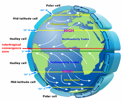
Another phenomenon that I came to know about through this project is how adjustments at the stratospheric level can shift the major air circulation cells. These six cells have distinct boundaries
and one of interest is the mid-latitude cell/arctic cell boundary. When this boundary shifts northward, it shifts a lot of warmer air over what was frozen ocean. When “global” warming
registers +1-2 degrees Celsius, it may be that +10-20 degrees were in one section of the Arctic. Such a large change requires a shift in a convection pattern to blow in the heat. Interestingly,
these pattern changes are not necessarily CO2-driven. There are publications that attribute such changes to stratospheric temperature, which is driven by ozone layer absorbance changes.
According to one study, when ozone layer is weaker, the stratosphere cools off and the mid-latitude cell boundary shifts northward into the arctic. □
Chris does chemical process development and overall design work in the chemical processing industry. Chris has 17 years of experience working with developing technology companies as well as
established chemical industries, which includes numerous international plant start-up assignments. Chris holds a BS in Chemical Engineering from the University of Michigan.
Some resources of interest:
Treatise on Thermodynamics by Max Planck (e-book)
The Theory of Heat Radiation by Max Planck (e-book)
Emissivity of a surface and the Leslie cube demonstration
NOAA Surface Radiation Budget Monitoring - how it's done
NOAA Global Monitoring Laboratory - greenhouse gasses
"Thinking About Climate" by Chemical Engineering Progress